Table Of Contents

Table Of Contents

13.11. 全卷积网络¶

如 13.9节中所介绍的那样，语义分割是对图像中的每个像素分类。 全卷积网络（fully convolutional network，FCN）采用卷积神经网络实现了从图像像素到像素类别的变换 (Long et al., 2015)。与我们之前在图像分类或目标检测部分介绍的卷积神经网络不同，全卷积网络将中间层特征图的高和宽变换回输入图像的尺寸：这是通过在 13.10节中引入的转置卷积（transposed convolution）实现的。因此，输出的类别预测与输入图像在像素级别上具有一一对应关系：通道维的输出即该位置对应像素的类别预测。

mindspore pytorch

%matplotlib inline
import os
import mindcv
import mindspore
from mindspore import nn, ops
from mindspore.ops import functional as F
from d2l import mindspore as d2l

%matplotlib inline
import os
import numpy as np
import torch
import torchvision
import torchvision.transforms.functional as TF
from PIL import Image
from torch import nn
from torch.nn import functional as F
from d2l import torch as d2l

13.11.1. 构造模型¶

下面我们了解一下全卷积网络模型最基本的设计。如图13.11.1所示，全卷积网络先使用卷积神经网络抽取图像特征，然后通过\(1\times 1\)卷积层将通道数变换为类别个数，最后在 13.10节中通过转置卷积层将特征图的高和宽变换为输入图像的尺寸。因此，模型输出与输入图像的高和宽相同，且最终输出通道包含了该空间位置像素的类别预测。

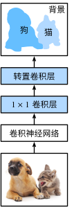
../_images/fcn.svg — 图13.11.1 全卷积网络¶

下面，我们使用在ImageNet数据集上预训练的ResNet-18模型来提取图像特征，并将该网络记为pretrained_net。 ResNet-18模型的最后几层包括全局平均汇聚层和全连接层，然而全卷积网络中不需要它们。

mindspore pytorch

pretrained_net = mindcv.create_model('resnet18', pretrained=True)
list(pretrained_net.cells())[-3:]

[SequentialCell(
   (0): BasicBlock(
     (conv1): Conv2d(input_channels=256, output_channels=512, kernel_size=(3, 3), stride=(2, 2), pad_mode=pad, padding=1, dilation=(1, 1), group=1, has_bias=False, weight_init=<mindspore.common.initializer.HeUniform object at 0x76dc46f5bdd0>, bias_init=None, format=NCHW)
     (bn1): BatchNorm2d(num_features=512, eps=1e-05, momentum=0.9, gamma=Parameter (name=layer4.0.bn1.gamma, shape=(512,), dtype=Float32, requires_grad=True), beta=Parameter (name=layer4.0.bn1.beta, shape=(512,), dtype=Float32, requires_grad=True), moving_mean=Parameter (name=layer4.0.bn1.moving_mean, shape=(512,), dtype=Float32, requires_grad=False), moving_variance=Parameter (name=layer4.0.bn1.moving_variance, shape=(512,), dtype=Float32, requires_grad=False))
     (relu): ReLU()
     (conv2): Conv2d(input_channels=512, output_channels=512, kernel_size=(3, 3), stride=(1, 1), pad_mode=pad, padding=1, dilation=(1, 1), group=1, has_bias=False, weight_init=<mindspore.common.initializer.HeUniform object at 0x76dc4a0bcf10>, bias_init=None, format=NCHW)
     (bn2): BatchNorm2d(num_features=512, eps=1e-05, momentum=0.9, gamma=Parameter (name=layer4.0.bn2.gamma, shape=(512,), dtype=Float32, requires_grad=True), beta=Parameter (name=layer4.0.bn2.beta, shape=(512,), dtype=Float32, requires_grad=True), moving_mean=Parameter (name=layer4.0.bn2.moving_mean, shape=(512,), dtype=Float32, requires_grad=False), moving_variance=Parameter (name=layer4.0.bn2.moving_variance, shape=(512,), dtype=Float32, requires_grad=False))
     (down_sample): SequentialCell(
       (0): Conv2d(input_channels=256, output_channels=512, kernel_size=(1, 1), stride=(2, 2), pad_mode=same, padding=0, dilation=(1, 1), group=1, has_bias=False, weight_init=<mindspore.common.initializer.HeUniform object at 0x76dc46f59ed0>, bias_init=None, format=NCHW)
       (1): BatchNorm2d(num_features=512, eps=1e-05, momentum=0.9, gamma=Parameter (name=layer4.0.down_sample.1.gamma, shape=(512,), dtype=Float32, requires_grad=True), beta=Parameter (name=layer4.0.down_sample.1.beta, shape=(512,), dtype=Float32, requires_grad=True), moving_mean=Parameter (name=layer4.0.down_sample.1.moving_mean, shape=(512,), dtype=Float32, requires_grad=False), moving_variance=Parameter (name=layer4.0.down_sample.1.moving_variance, shape=(512,), dtype=Float32, requires_grad=False))
     )
   )
   (1): BasicBlock(
     (conv1): Conv2d(input_channels=512, output_channels=512, kernel_size=(3, 3), stride=(1, 1), pad_mode=pad, padding=1, dilation=(1, 1), group=1, has_bias=False, weight_init=<mindspore.common.initializer.HeUniform object at 0x76dc46f700d0>, bias_init=None, format=NCHW)
     (bn1): BatchNorm2d(num_features=512, eps=1e-05, momentum=0.9, gamma=Parameter (name=layer4.1.bn1.gamma, shape=(512,), dtype=Float32, requires_grad=True), beta=Parameter (name=layer4.1.bn1.beta, shape=(512,), dtype=Float32, requires_grad=True), moving_mean=Parameter (name=layer4.1.bn1.moving_mean, shape=(512,), dtype=Float32, requires_grad=False), moving_variance=Parameter (name=layer4.1.bn1.moving_variance, shape=(512,), dtype=Float32, requires_grad=False))
     (relu): ReLU()
     (conv2): Conv2d(input_channels=512, output_channels=512, kernel_size=(3, 3), stride=(1, 1), pad_mode=pad, padding=1, dilation=(1, 1), group=1, has_bias=False, weight_init=<mindspore.common.initializer.HeUniform object at 0x76dc46f58650>, bias_init=None, format=NCHW)
     (bn2): BatchNorm2d(num_features=512, eps=1e-05, momentum=0.9, gamma=Parameter (name=layer4.1.bn2.gamma, shape=(512,), dtype=Float32, requires_grad=True), beta=Parameter (name=layer4.1.bn2.beta, shape=(512,), dtype=Float32, requires_grad=True), moving_mean=Parameter (name=layer4.1.bn2.moving_mean, shape=(512,), dtype=Float32, requires_grad=False), moving_variance=Parameter (name=layer4.1.bn2.moving_variance, shape=(512,), dtype=Float32, requires_grad=False))
   )
 ),
 GlobalAvgPooling(),
 Dense(input_channels=512, output_channels=1000, has_bias=True)]

pretrained_net = torchvision.models.resnet18(pretrained=True)
list(pretrained_net.children())[-3:]

[Sequential(
   (0): BasicBlock(
     (conv1): Conv2d(256, 512, kernel_size=(3, 3), stride=(2, 2), padding=(1, 1), bias=False)
     (bn1): BatchNorm2d(512, eps=1e-05, momentum=0.1, affine=True, track_running_stats=True)
     (relu): ReLU(inplace=True)
     (conv2): Conv2d(512, 512, kernel_size=(3, 3), stride=(1, 1), padding=(1, 1), bias=False)
     (bn2): BatchNorm2d(512, eps=1e-05, momentum=0.1, affine=True, track_running_stats=True)
     (downsample): Sequential(
       (0): Conv2d(256, 512, kernel_size=(1, 1), stride=(2, 2), bias=False)
       (1): BatchNorm2d(512, eps=1e-05, momentum=0.1, affine=True, track_running_stats=True)
     )
   )
   (1): BasicBlock(
     (conv1): Conv2d(512, 512, kernel_size=(3, 3), stride=(1, 1), padding=(1, 1), bias=False)
     (bn1): BatchNorm2d(512, eps=1e-05, momentum=0.1, affine=True, track_running_stats=True)
     (relu): ReLU(inplace=True)
     (conv2): Conv2d(512, 512, kernel_size=(3, 3), stride=(1, 1), padding=(1, 1), bias=False)
     (bn2): BatchNorm2d(512, eps=1e-05, momentum=0.1, affine=True, track_running_stats=True)
   )
 ),
 AdaptiveAvgPool2d(output_size=(1, 1)),
 Linear(in_features=512, out_features=1000, bias=True)]

接下来，我们创建一个全卷积网络net。它复制了ResNet-18中大部分的预训练层，除了最后的全局平均汇聚层和最接近输出的全连接层。

mindspore pytorch

net = nn.SequentialCell(*list(pretrained_net.cells())[:-2])

net = nn.Sequential(*list(pretrained_net.children())[:-2])

给定高度为320和宽度为480的输入，net的前向传播将输入的高和宽减小至原来的\(1/32\)，即10和15。

mindspore pytorch

X = ops.rand((1, 3, 320, 480))
net(X).shape

(1, 512, 10, 15)

X = torch.rand(size=(1, 3, 320, 480))
net(X).shape

torch.Size([1, 512, 10, 15])

接下来使用\(1\times1\)卷积层将输出通道数转换为Pascal VOC2012数据集的类数（21类）。最后需要将特征图的高度和宽度增加32倍，从而将其变回输入图像的高和宽。回想一下 6.3节中卷积层输出形状的计算方法：由于\((320-64+16\times2+32)/32=10\)且\((480-64+16\times2+32)/32=15\)，我们构造一个步幅为\(32\)的转置卷积层，并将卷积核的高和宽设为\(64\)，填充为\(16\)。我们可以看到如果步幅为\(s\)，填充为\(s/2\)（假设\(s/2\)是整数）且卷积核的高和宽为\(2s\)，转置卷积核会将输入的高和宽分别放大\(s\)倍。

mindspore pytorch

num_classes = 21
net = nn.SequentialCell(*list(pretrained_net.cells())[:-2],
                        nn.Conv2d(512, num_classes, kernel_size=1),
                        nn.Conv2dTranspose(num_classes, num_classes,
                                    kernel_size=64, padding=16, stride=32, pad_mode='pad')
                       )

num_classes = 21
net.add_module('final_conv', nn.Conv2d(512, num_classes, kernel_size=1))
net.add_module('transpose_conv', nn.ConvTranspose2d(num_classes, num_classes,
                                    kernel_size=64, padding=16, stride=32))

13.11.2. 初始化转置卷积层¶

在图像处理中，我们有时需要将图像放大，即上采样（upsampling）。 双线性插值（bilinear interpolation）是常用的上采样方法之一，它也经常用于初始化转置卷积层。

为了解释双线性插值，假设给定输入图像，我们想要计算上采样输出图像上的每个像素。

将输出图像的坐标\((x,y)\)映射到输入图像的坐标\((x',y')\)上。例如，根据输入与输出的尺寸之比来映射。请注意，映射后的\(x′\)和\(y′\)是实数。
在输入图像上找到离坐标\((x',y')\)最近的4个像素。
输出图像在坐标\((x,y)\)上的像素依据输入图像上这4个像素及其与\((x',y')\)的相对距离来计算。

双线性插值的上采样可以通过转置卷积层实现，内核由以下bilinear_kernel函数构造。限于篇幅，我们只给出bilinear_kernel函数的实现，不讨论算法的原理。

mindspore pytorch

def bilinear_kernel(in_channels, out_channels, kernel_size):
    factor = (kernel_size + 1) // 2
    if kernel_size % 2 == 1:
        center = factor - 1
    else:
        center = factor - 0.5
    og = (ops.arange(kernel_size).reshape(-1, 1),
          ops.arange(kernel_size).reshape(1, -1))
    filt = (1 - ops.abs(og[0] - center) / factor) * \
           (1 - ops.abs(og[1] - center) / factor)
    weight = ops.zeros((in_channels, out_channels,
                          kernel_size, kernel_size))
    weight[list(range(in_channels)), list(range(out_channels)), :, :] = filt
    return weight

def bilinear_kernel(in_channels, out_channels, kernel_size):
    factor = (kernel_size + 1) // 2
    if kernel_size % 2 == 1:
        center = factor - 1
    else:
        center = factor - 0.5
    og = (torch.arange(kernel_size).reshape(-1, 1),
          torch.arange(kernel_size).reshape(1, -1))
    filt = (1 - torch.abs(og[0] - center) / factor) * \
           (1 - torch.abs(og[1] - center) / factor)
    weight = torch.zeros((in_channels, out_channels,
                          kernel_size, kernel_size))
    weight[range(in_channels), range(out_channels), :, :] = filt
    return weight

让我们用双线性插值的上采样实验它由转置卷积层实现。我们构造一个将输入的高和宽放大2倍的转置卷积层，并将其卷积核用bilinear_kernel函数初始化。

mindspore pytorch

conv_trans = nn.Conv2dTranspose(3, 3, kernel_size=4, padding=1, stride=2, pad_mode='pad',
                                has_bias=False)
conv_trans.weight.set_data(bilinear_kernel(3, 3, 4));

conv_trans = nn.ConvTranspose2d(3, 3, kernel_size=4, padding=1, stride=2,
                                bias=False)
conv_trans.weight.data.copy_(bilinear_kernel(3, 3, 4));

读取图像X，将上采样的结果记作Y。为了打印图像，我们需要调整通道维的位置。

mindspore pytorch

img = mindspore.dataset.vision.ToTensor()(d2l.Image.open('../img/catdog.jpg'))
img = mindspore.Tensor(img)
X = img.unsqueeze(0)
Y = conv_trans(X)
out_img = Y[0].permute(1, 2, 0)

img = torchvision.transforms.ToTensor()(d2l.Image.open('../img/catdog.jpg'))
X = img.unsqueeze(0)
Y = conv_trans(X)
out_img = Y[0].permute(1, 2, 0).detach()

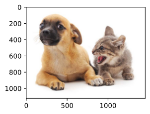
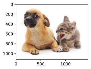
可以看到，转置卷积层将图像的高和宽分别放大了2倍。除了坐标刻度不同，双线性插值放大的图像和在 13.3节中打印出的原图看上去没什么两样。

mindspore pytorch

d2l.set_figsize()
print('input image shape:', img.permute(1, 2, 0).shape)
d2l.plt.imshow(img.permute(1, 2, 0).numpy());
print('output image shape:', out_img.shape)
d2l.plt.imshow(out_img.numpy());

input image shape: (561, 728, 3)
output image shape: (1122, 1456, 3)

../_images/output_fcn_ce3435_75_1.svg

d2l.set_figsize()
print('input image shape:', img.permute(1, 2, 0).shape)
d2l.plt.imshow(img.permute(1, 2, 0));
print('output image shape:', out_img.shape)
d2l.plt.imshow(out_img);

input image shape: torch.Size([561, 728, 3])
output image shape: torch.Size([1122, 1456, 3])

../_images/output_fcn_ce3435_78_1.svg

全卷积网络用双线性插值的上采样初始化转置卷积层。对于\(1\times 1\)卷积层，我们使用Xavier初始化参数。

mindspore pytorch

W = bilinear_kernel(num_classes, num_classes, 64)
net[-1].weight.set_data(W);

W = bilinear_kernel(num_classes, num_classes, 64)
net.transpose_conv.weight.data.copy_(W);

13.11.3. 读取数据集¶

我们用 13.9节中介绍的语义分割读取数据集。指定随机裁剪的输出图像的形状为\(320\times 480\)：高和宽都可以被\(32\)整除。

mindspore pytorch

batch_size, crop_size = 32, (320, 480)
train_iter, test_iter = d2l.load_data_voc(batch_size, crop_size)

read 1114 examples
read 1078 examples

batch_size, crop_size = 32, (320, 480)
train_iter, test_iter = d2l.load_data_voc(batch_size, crop_size)

read 1114 examples
read 1078 examples

13.11.4. 训练¶

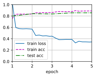
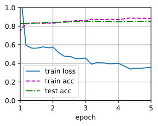
现在我们可以训练全卷积网络了。这里的损失函数和准确率计算与图像分类中的并没有本质上的不同，因为我们使用转置卷积层的通道来预测像素的类别，所以需要在损失计算中指定通道维。此外，模型基于每个像素的预测类别是否正确来计算准确率。

mindspore pytorch

def loss(inputs, targets):
    return F.cross_entropy(inputs, targets, reduction='none').mean(1).mean(1)

num_epochs, lr, wd = 5, 0.002, 1e-3
trainer = nn.SGD(net.trainable_params(), learning_rate=lr, weight_decay=wd)
d2l.train_ch13(net, train_iter, test_iter, loss, trainer, num_epochs)

loss 0.344, train acc 0.888, test acc 0.856
276.4 examples/sec on GPU

../_images/output_fcn_ce3435_102_1.svg

def loss(inputs, targets):
    return F.cross_entropy(inputs, targets, reduction='none').mean(1).mean(1)

num_epochs, lr, wd, devices = 5, 0.002, 1e-3, d2l.try_all_gpus()
trainer = torch.optim.SGD(net.parameters(), lr=lr, weight_decay=wd)
d2l.train_ch13(net, train_iter, test_iter, loss, trainer, num_epochs, devices)

loss 0.357, train acc 0.883, test acc 0.854
479.1 examples/sec on [device(type='cuda', index=0)]

../_images/output_fcn_ce3435_105_1.svg

13.11.5. 预测¶

在预测时，我们需要将输入图像在各个通道做标准化，并转成卷积神经网络所需要的四维输入格式。

mindspore pytorch

transform = mindspore.dataset.vision.Normalize(
            mean=[0.485, 0.456, 0.406], std=[0.229, 0.224, 0.225])

def normalize_image(img):
    return transform(img.astype('float32') / 255)

def predict(img):
    X = mindspore.Tensor(normalize_image(img).transpose(2, 0, 1)).unsqueeze(0)
    pred = net(X).argmax(axis=1)
    return pred.reshape(pred.shape[1], pred.shape[2])

transform = torchvision.transforms.Normalize(
    mean=[0.485, 0.456, 0.406], std=[0.229, 0.224, 0.225])

def normalize_image(img):
    img = torch.tensor(img, dtype=torch.float32).permute(2, 0, 1) / 255.0
    return transform(img)

def predict(img):
    X = normalize_image(img).unsqueeze(0)
    net.eval()
    with torch.no_grad():
        pred = net(X.to(devices[0])).argmax(dim=1)
    return pred.reshape(pred.shape[1], pred.shape[2]).cpu()

为了可视化预测的类别给每个像素，我们将预测类别映射回它们在数据集中的标注颜色。

mindspore pytorch

colormap = mindspore.Tensor(d2l.VOC_COLORMAP)

def label2image(pred):
    X = pred.long()
    return colormap[X, :]

colormap = torch.tensor(d2l.VOC_COLORMAP, dtype=torch.uint8)

def label2image(pred):
    X = pred.long().cpu()
    return colormap[X, :]

测试数据集中的图像大小和形状各异。由于模型使用了步幅为32的转置卷积层，因此当输入图像的高或宽无法被32整除时，转置卷积层输出的高或宽会与输入图像的尺寸有偏差。为了解决这个问题，我们可以在图像中截取多块高和宽为32的整数倍的矩形区域，并分别对这些区域中的像素做前向传播。请注意，这些区域的并集需要完整覆盖输入图像。当一个像素被多个区域所覆盖时，它在不同区域前向传播中转置卷积层输出的平均值可以作为softmax运算的输入，从而预测类别。

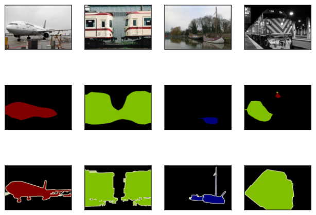
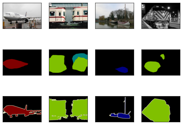
为简单起见，我们只读取几张较大的测试图像，并从图像的左上角开始截取形状为\(320\times480\)的区域用于预测。对于这些测试图像，我们逐一打印它们截取的区域，再打印预测结果，最后打印标注的类别。

mindspore pytorch

voc_dir = d2l.download_extract('voc2012', 'VOCdevkit/VOC2012')
test_images, test_labels = d2l.read_voc_images(voc_dir, False)

n, imgs = 4, []
for i in range(n):
    crop_rect = (0, 0, 320, 480)

    # 加载图像
    img = mindspore.dataset.vision.read_image(os.path.join(
        voc_dir, 'JPEGImages', f'{test_images[i]}.jpg'))
    label = mindspore.dataset.vision.read_image(os.path.join(
        voc_dir, 'SegmentationClass', f'{test_labels[i]}.png'))

    X = d2l.crop(img, *crop_rect)
    pred = label2image(predict(X))
    imgs += [X, pred.numpy(),
             d2l.crop(label, *crop_rect)]

d2l.show_images(imgs[::3] + imgs[1::3] + imgs[2::3], 3, n, scale=2);

../_images/output_fcn_ce3435_129_0.svg

voc_dir = d2l.download_extract('voc2012', 'VOCdevkit/VOC2012')
test_images, test_labels = d2l.read_voc_images(voc_dir, False)

n, imgs = 4, []
for i in range(n):
    crop_rect = (0, 0, 320, 480)

    img = np.array(Image.open(os.path.join(
        voc_dir, 'JPEGImages', f'{test_images[i]}.jpg')).convert('RGB'))
    label_rgb_raw = np.array(Image.open(os.path.join(
        voc_dir, 'SegmentationClass', f'{test_labels[i]}.png')).convert('RGB'))
    X = img[crop_rect[0]:crop_rect[0]+crop_rect[2],
            crop_rect[1]:crop_rect[1]+crop_rect[3], :]
    pred_np = label2image(predict(X)).numpy()
    img_show = X
    label_crop = label_rgb_raw[crop_rect[0]:crop_rect[0]+crop_rect[2],
                               crop_rect[1]:crop_rect[1]+crop_rect[3]]
    imgs += [img_show, pred_np, label_crop]

d2l.show_images(imgs[::3] + imgs[1::3] + imgs[2::3], 3, n, scale=2);

../_images/output_fcn_ce3435_132_0.svg

13.11.6. 小结¶

全卷积网络先使用卷积神经网络抽取图像特征，然后通过\(1\times 1\)卷积层将通道数变换为类别个数，最后通过转置卷积层将特征图的高和宽变换为输入图像的尺寸。
在全卷积网络中，我们可以将转置卷积层初始化为双线性插值的上采样。

13.11.7. 练习¶

如果将转置卷积层改用Xavier随机初始化，结果有什么变化？
调节超参数，能进一步提升模型的精度吗？
预测测试图像中所有像素的类别。
最初的全卷积网络的论文中 (Long et al., 2015)还使用了某些卷积神经网络中间层的输出。试着实现这个想法。

mindspore pytorch

Table Of Contents

13.11. 全卷积网络

13.10. 转置卷积

13.12. 风格迁移